ANOVA
Pre-Class Readings and Videos
In our description of hypothesis testing in the previous chapter, we started with case C→Q, where the explanatory variable/independent variable/predictor (X = major depression) is categorical and the response variable/dependent variable/outcome (Y = number of cigarettes smoked) is quantitative. Here is a similar example:
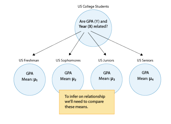
GPA and Year in College
Say that our variable of interest is the GPA of college students in the United States. Since GPA is quantitative, we do inference on µ, the (population) mean GPA among all U.S. college students. We are really interested in the relationship between GPA and college year:
- X : year in college (1 = freshmen, 2 = sophomore, 3 = junior, 4 = senior)
- Y : GPA
In other words, we want to explore whether GPA is related to year in college. The way to think about this is that the population of U.S. college students is now broken into 4 subpopulations: freshmen, sophomores, juniors, and seniors. Within each of these four groups, we are interested in the GPA.
The inference must therefore involve the 4 sub-population means:
- µ1 : mean GPA among freshmen in the United States
- µ2 : mean GPA among sophomores in the United States
- µ3 : mean GPA among juniors in the United States
- µ4 : mean GPA among seniors in the United States
It makes sense that the inference about the relationship between year and GPA has to be based on some kind of comparison of these four means. If we infer that these four means are not all equal (i.e., that there are some differences in GPA across years in college) then that’s equivalent to saying GPA is related to year in college. Let’s summarize this example with a figure:
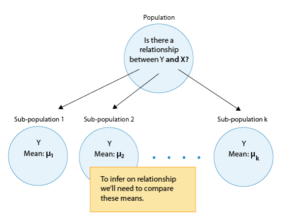
In general, then, making inferences about the relationship between X and Y in Case C→Q boils down to comparing the means of Y in the sub-populations, which are created by the categories defined in X (say k categories). The following figure summarizes this:
The inferential method for comparing means is called Analysis of Variance (abbreviated as ANOVA), and the test associated with this method is called the ANOVA F-test. We will first present our leading example, and then introduce the ANOVA F-test by going through its 4 steps, illustrating each one using the example.
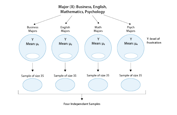
Is “academic frustration” related to major?
A college dean believes that students with different majors may experience different levels of academic frustration. Random samples of size 35 of Business, English, Mathematics, and Psychology majors are asked to rate their level of academic frustration on a scale of 1 (lowest) to 20 (highest)
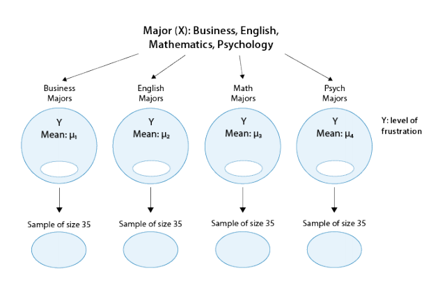
The figure highlights that examining the relationship between major (X) and frustration level (Y) amounts to comparing the mean frustration levels (µ1,µ2,µ3,µ4) among the four majors defined by X.
The Anova F-Test
Now that we understand in what kind of situations ANOVA is used, we are ready to learn how it works.
Stating the Hypotheses
The null hypothesis claims that there is no relationship between X and Y. Since the relationship is examined by comparing µ1,µ2,µ3,…µk (the means of Y in the populations defined by the values of X), no relationship would mean that all the means are equal. Therefore the null hypothesis of the F-test is: H0:µ1=µ2=…=µk.
As we mentioned earlier, here we have just one alternative hypothesis, which claims that there is a relationship between X and Y. In terms of the means µ1,µ2,µ3,…,µk, it simply says the opposite of the alternative, that not all the means are equal, and we simply write: Ha: not all the µ′s are equal.
Recall our “Is academic frustration related to major?” example:
The correct hypotheses for our example are:
- H0: µ1=µ2=µ3=µ4
- HA: Not all µi’s are the same
Note that there are many ways for µ1,µ2,µ3,µ4 not to be all equal, and µ1≠µ2≠µ3≠µ4 is just one of them. Another way could be µ1=µ2=µ3≠µ4 or µ1=µ2≠µ3=µ4. The alternative of the ANOVA F-test simply states that not all of the means are equal and is not specific about the way in which they are different.
The Idea Behind the ANOVA F-Test
Let’s think about how we would go about testing whether the population means µ1,µ2,µ3,µ4 are equal. It seems as if the best we could do is to calculate their point estimates—the sample mean in each of our 4 samples (denote them by ȳ1,ȳ2,ȳ3,ȳ4), and see how far apart these sample means are, or, in other words, measure the variation between the sample means. If we find that the four sample means are not all close together, we’ll say that we have evidence against Ho, and otherwise, if they are close together, we’ll say that we do not have evidence against Ho. This seems quite simple, but is this enough? Let’s see.
It turns out that:
- The sample mean frustration score of the 35 business majors is: ȳ1 = 7.3
- The sample mean frustration score of the 35 English majors is: ȳ2= 1.8
- The sample mean frustration score of the 35 math majors is: ȳ3= 3.2
- The sample mean frustration score of the 35 psychology majors is: ȳ4= 4.0
Below we present two possible scenarios for our example. In both cases, we construct side-by-side box plots (showing the distribution of the data including the range, lowest and highest values, the median, mean, etc.) for each of the four groups on frustration level. Scenario #1 and Scenario #2 both show data for four groups with the sample means 7.3, 11.8, 13.2, and 14.0 (means indicated with red marks).
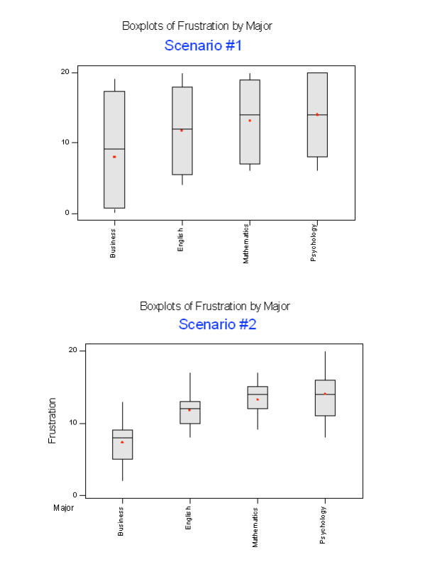
The important difference between the two scenarios is that the first represents data with a large amount of variation within each of the four groups; the second represents data with a small amount of variation within each of the four groups.
Scenario 1, because of the large amount of spread within the groups, shows box plots with plenty of overlap. One could imagine the data arising from 4 random samples taken from 4 populations, all having the same mean of about 11 or 12. The first group of values may have been a bit on the low side, and the other three a bit on the high side, but such differences could conceivably have come about by chance. This would be the case if the null hypothesis, claiming equal population means, were true. Scenario 2, because of the small amount of spread within the groups, shows boxplots with very little overlap. It would be very hard to believe that we are sampling from four groups that have equal population means. This would be the case if the null hypothesis, claiming equal population means, were false.
Thus, in the language of hypothesis tests, we would say that if the data were configured as they are in scenario 1, we would not reject the null hypothesis that population mean frustration levels were equal for the four majors. If the data were configured as they are in scenario 2, we would reject the null hypothesis, and we would conclude that mean frustration levels differ depending on major.
Let’s summarize what we learned from this. The question we need to answer is: Are the differences among the sample means ( ȳ’s) due to true differences among the µ’s (alternative hypothesis), or merely due to sampling variability (null hypothesis)?
In order to answer this question using our data, we obviously need to look at the variation among the sample means, but this alone is not enough. We need to look at the variation among the sample means relative to the variation within the groups. In other words, we need to look at the quantity:
- Variation among sample means / Variation within groups
which measures to what extent the difference among the sampled groups’ means dominates over the usual variation within the sampled groups (which reflects differences in individuals that are typical in random samples).
When the variation within groups is large (like in scenario 1), the variation (differences) among the sample means could become negligible and the data provide very little evidence against Ho.When the variation within groups is small (like in scenario 2), the variation among the sample means dominates over it, and the data have stronger evidence against Ho.
Looking at this ratio of variations is the idea behind the comparison of means; hence the name analysis of variance (ANOVA).
Did I Get This?
Suppose we are investigating interview scores for an executive level position where applicants are rated from 0 (not at all qualified) to 50 (extremely qualified). We want to investigate the effectiveness of 3 interview training programs (which we will denote — program 1, program 2, and program 3. Ultimately we would like to know whether there is an association between training program and interview scores. That is, we would like to test the hypothesis:
- H0: µ1=µ2=µ3
- HA: Not all µi’s are the same
The following are two possible scenarios of the data (note in both scenarios the sample means are 25, 30, and 35).
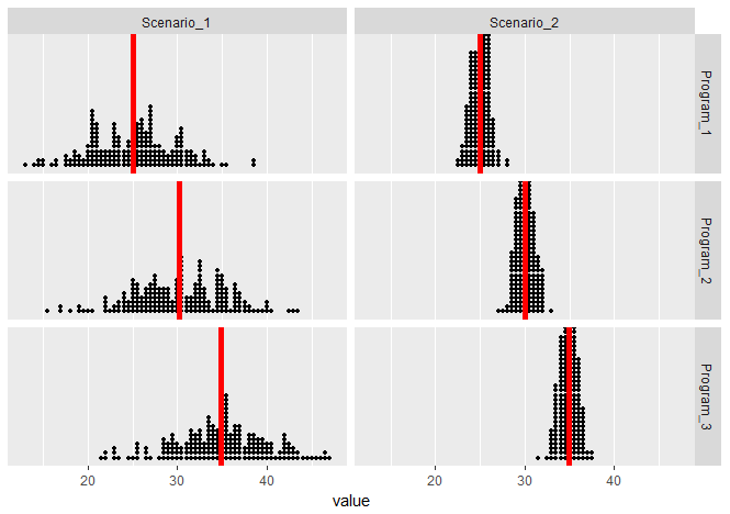
In both scenarios (since the means are the same), we have the same between group variation. But these scenarios vary greatly on their within group variation — notice that the within group variation is visibly smaller in Scenario 2 than it is in Scenario 1. Both scenarios seem to visually imply there is a relationship between Program and Interview Score, but the evidence in Scenario 2 is more compelling.
Finding the P-Value
The p-value of the ANOVA F-test is the probability of getting an F statistic as large as we got (or even larger) had H0:µ1=µ2=…=µk been true. In other words, it tells us how surprising it is to find data like those observed, assuming that there is no difference among the population means µ1, µ2, …,µk.
Returning back to our example of Academic Frustration and Major, we can obtain the following output using R, SAS, or STATA (there should be only small variations between them):
| Df | Sum Sq. | Mean Sq. | F-value | P-value | |
| Major | 3 | 939.85 | 313.28 | 46.601 | <2.2e-16 |
| Residuals | 136 | 914.29 | 6.72 |
The p-value in this example is so small that it is essentially 0, telling us that it would be next to impossible to get data like those observed had the mean frustration level of the four majors been the same (as the null hypothesis claims).
Making Conclusions in Context
As usual, we base our conclusion on the p-value. A small p-value tells us that our data contain evidence against Ho. More specifically, a small p-value tells us that the differences between the sample means are statistically significant (unlikely to have happened by chance), and therefore we reject Ho. If the p-value is not small, the data do not provide enough evidence to reject Ho, and so we continue to believe that it may be true. A significance level (cut-off probability) of .05 can help determine what is considered a small p-value.
In our example, the p-value is extremely small (close to 0) indicating that our data provide extremely strong evidence to reject Ho. We conclude that the frustration level means of the four majors are not all the same, or, in other words, that majors are related to students’ academic frustration levels at the school where the test was conducted.
Post Hoc Tests
When testing the relationship between your explanatory (X) and response variable (Y) in the context of ANOVA, your categorical explanatory variable (X) may have more than two levels.
For example, when we examine the differences in mean GPA (Y) across different college years (X=freshman, sophomore, junior and senior) or the differences in mean frustration level (Y) by college major (X=Business, English, Mathematics, Psychology), there is just one alternative hypothesis, which claims that there is a relationship between X and Y.
In terms of the means µ1,µ2,µ3,…,µk,(ANOVA), it simply says the opposite of the alternative, that not all the means are equal.
Example:
Note that there are many ways for µ1,µ2,µ3,µ4 not to be all equal, and µ1≠µ2≠µ3≠µ4 is just one of them. Another way could be µ1=µ2=µ3≠µ4 or µ1=µ2≠µ3=µ4.
In the case where the explanatory variable (X) represents more than two groups, a significant ANOVA F test does not tell us which groups are different from the others.
To determine which groups are different from the others, we would need to perform post hoc tests. These tests, done after the ANOVA, are generally termed post hoc paired comparisons.
Post hoc paired comparisons (meaning “after the fact” or “after data collection”) must be conducted in a particular way in order to prevent excessive Type I error.
Type I error occurs when you make an incorrect decision about the null hypothesis. Specifically, this type of error is made when your p-value makes you reject the null hypothesis (H0) when it is true. In other words, your p-value is sufficiently small for you to say that there is a real association, despite the fact that the differences you see are due to chance alone. The type I error rate equals your p-value and is denoted by the Greek letter α (alpha).
Although a Type I Error rate of .05 is considered acceptable (i.e. it is acceptable that 5 times out of 100 you will reject the null hypothesis when it is true), higher Type I error rates are not considered acceptable. If you were to use the significance level of .05 across multiple paired comparisons (for example, three) with p = .05, then the p rate across all three comparisons is .05+.05+.05, or .15, yielding a 15% Type I Error rate. In other words, across the unprotected paired comparisons you will reject the null hypothesis when it is true, 15 times out of 100.
The purpose of running protected post hoc tests is that they allow you to conduct multiple paired comparisons without inflating the Type I Error rate.
For ANOVA, you can use one of several post hoc tests, each which control for Type I Error, while performing paired comparisons (Duncan Multiple Range test, Dunnett’s Multiple Comparison test, Newman-Keuls test, Scheffe’s test, Tukey’s HSD test, Fisher’s LSD test, Sidak).
Please watch the videos below:
- R
- SAS
- Stata
Pre-Class Quiz
After reviewing the material above, take Quiz 8 (click here). Please note that you have 2 attempts for this quiz and the higher grade prevails.
During Class Tasks
Mini-Assignment 5
Project Component H (if applicable)
Codebooks and Data ArchitectureLiterature Review
Working with DataData Management
Graphing VariablesGraphing Releationships
Hypothesis Testing and ANOVAChi-square and Correlation
Exploring Third VariablesExam 2
Regression and Study DesignConfounding and Multivariate Models